Imagine for some reason, two of your favorite songs are playing on two different speakers, at different volumes, one louder than the other. There is a likely chance that you will involuntarily vibe to the louder song, why? Because it is louder.

Similarly, Machine Learning algorithms behave the same way when training on data where two classes occur disproportionately. Because the 0s or NOs occur more frequently than the 1s or YESs, the algorithm pays more attention to the NOs during training, and will end up predicting "NO" for a new data point, when the correct outcome might actually be "YES". This is a situation you wouldn't want, especially if your algorithm is heavily relied upon for direction by business stakeholders.

Thankfully, there are a number of techniques that can help rectify this kind of situation (Class Imbalance). One is over-sampling and undersampling of the majority and minority classes respectively.

For the purpose of this tutorial, we will be focusing on a combination of class weight balancing and ensemble learning.

Prerequisites

This tutorial is intended for a mid-level audience. But you can follow through if you have:

• Some experience with predictive modeling
• Intermediate use of the Python Programming Language
• An understanding of the classification technique in Machine Learning.

Definition of terms used in this tutorial

• Class: A class refers to a type of outcome in a dataset, and it is quite useful in training classifiers to categorize instances of data. In a binary classification problem, a class can be Yes/No, 1 or 0, True or False. In a Multi-classification problem, it can be 1,2,3,4 or 5.
• Classification: A technique in machine learning that involves categorizing observations or rows in a dataset into classes. You can revisit the example I gave above to aid your understanding.
• Predictive Modeling: A method used in Machine Learning and Data Science to forecast or predict future outcomes with past occurrences.
• Algorithm: Machine Learning algorithms are simply a set of rules, driven by maths and logic, which are able to learn patterns from data.
• Learning: A process by which an algorithm acquires, and adapts to new information with little human intervention.
• Weight: You can think of weight as the importance of a datapoint. This could be a feature or even a class.
• Decision Tree: A decision tree is an algorithm that helps us come to a conclusion or prediction (in this case), by asking questions about the data in a sequential manner. When applied to a binary classification problem, each question asked by a decision tree leads to either a yes or no, answer, which is now broken further down by another question.
• Logistic Regression: In simple terms, Logistic Regression is a mathematical algorithm that measures the cause and effect between two types of variables (independent and dependent variables). It also predicts binary outcomes by computing a weighted sum of independent features.

However, this list is not exhaustive. You'll come across terms not defined above as we go further along. Hyperlinks for further reading have been attached to the terms.

Class Weights and Balancing?

Sequel to the introduction, imbalanced data causes an algorithm to apply unequal importance to classes based on how frequently they occur. And so, the class that occurs more frequently has more of the algorithm's attention, compared to the infrequent class.

A simple solution might be refocusing the algorithm's attention, such that it lays more importance on the infrequent class. This process is called class weight balancing.

Re-ascribing the importance an algorithm places on either class is guided by the following formula

W_j = N /(K * n_j)

Where:

• W_j: The weight of a class
• N: The Number of rows in the data
• K: The number of classes
• n_j: The number of observations of J^th class

With this logic, the weight of a class will be inversely proportional to its frequency within the data. And so, the lower the number of observations of a particular class, the more important that class will be to the algorithm. Let’s test out this logic on a sample dataset.

An Example

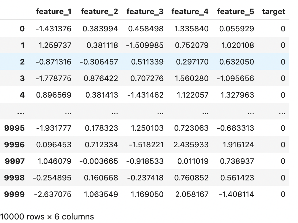
We create a dummy dataset of 10,000 rows with a class imbalance of 90:10 (90% of observations for class 0, and 10% of observations for class 1) with this line of code:

import pandas as pd
from sklearn.datasets import make_classification
X, y = make_classification(n_samples = 10000,
                           n_features = 5,
                           n_informative = 3,
                           n_classes = 2,
                           weights = [0.90, 0.10])

data = pd.DataFrame(X, columns = ['feature_1', 'feature_2', 'feature_3', 'feature_4', 'feature_5'])
data['target'] = y

In this conjured data, we have 5 independent features and 1 target feature. The majority class is 0 and the minority class is 1. This exemplifies the kind of situation you might experience when dealing with fraud detection, heart disease prediction, etc.

If we train an algorithm with this data, chances are that it may not have a decent performance when identifying true positives, or in this case 1s. Let’s test this idea out by training a simple Logistic Regression algorithm.

from sklearn.metrics import confusion_matrix
import matplotlib.pyplot as plt
import seaborn as sns
from sklearn.linear_model import LogisticRegression
from sklearn.model_selection import train_test_split
log_reg = LogisticRegression()

def compute_metrics(y_test, y_pred):
    cm = pd.DataFrame(confusion_matrix(y_test, y_pred))
    plt.figure(figsize=(4, 2))
    sns.heatmap(cm, annot=True, fmt='g')
    plt.title('Confusion Matrix')
    plt.ylabel('Actual Values')
    plt.xlabel('Predicted Values')
    plt.show()

x_train, x_test, y_train, y_test = train_test_split(X, y, stratify = y)

log_reg.fit(x_train, y_train)
y_pred = log_reg.predict(x_test)

compute_metrics(y_test, y_pred)

Here we are splitting the data into train and test sets, both containing 7,500 and 2,500 records respectively. We are also fitting a Logistic Regression algorithm on the train set and evaluating the algorithm on the test set. The algorithm's performance is visualized with a confusion matrix that can be seen below

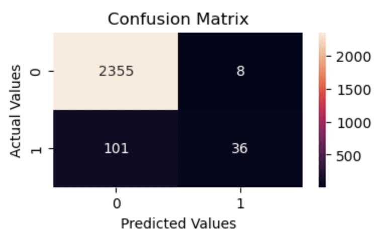
The classifier has no trouble recognizing a negative instance, as we can see the negative class has 2,355 instances that are correctly classified. We however cannot say the same for the positive instance.

Observations that are truly positive but categorized as negative (False Negatives) are 101, and observations that are positive and correctly classified as such (True Positives) are 36.

To put this in perspective, out of 137 positive instances in the test set, 36 were classified correctly and 101 were classified wrongly.

Now, let’s balance the class weights by making them inversely proportional to the number of observations for each class. The scikit-learn library used here has a parameter for most classification algorithms called class_weight parameter that allows you to specify or balance out the weights of classes.

log_reg = LogisticRegression(class_weight = 'balanced', 
solver = 'liblinear')

log_reg.fit(x_train, y_train)
y_pred = log_reg.predict(x_test)

precision_score(y_test, y_pred)
compute_metrics(y_test, y_pred)

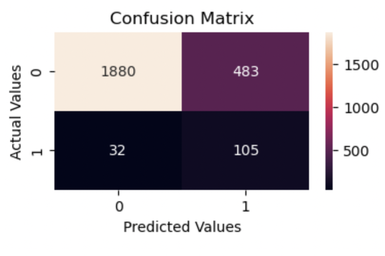
On the first look, we see that the True Positives have increased to 105 from 101 and False Negatives have reduced to 32 from 36.

But not so fast, the False Positives have increased to 483 from 8, and so we have another challenge to deal with. Perhaps we might have tipped the class weight in favor of the minority set so much so that it is not learning the observations of the majority class properly.

So a new question comes up.

How can we improve the algorithm's performance?

1. We could iterate over some values to find the right combination of weights that does not deny the negative class of the algorithm’s attention. This is repetitive and may take a while before we arrive at that combination.

2. We could also train a number of algorithms on the data and combine them by aggregating their predictions to give a final prediction. This is something that many literature call Ensemble Learning. It is very similar to a situation where the aggregated answers of many random people point to the right direction on a subject matter compared to the opinion of one person.

Ensemble Learning

Ensemble learning is a technique in Machine Learning premised on the idea that classifiers combined together, offer better predictive performance than a single classifier, even if the classifiers are individually weak. The solutions to the Netflix Prize Competition of 2009 attest to this.

Primarily, there are three main methods of ensemble learning:

• Bagging
• Boosting
• Stacking

Bagging: A variant of ensemble learning where different classification algorithms are trained on the same data and their predictions are aggregated together to give a final prediction. Conversely, it is possible to train the same algorithm on different subsets of the data and still achieve a bagging ensemble method. A great example of a Bagging classifier is the Random Forest Classifier as we will see shortly.

Boosting: Another approach to Ensemble learning is boosting. Otherwise called hypothesis boosting, the boosting method involves training classifiers to arrive at a stronger prediction. However, training these classifiers is done sequentially. In clearer terms classifiers are trained in a sequential manner, with each classifier trained to correct the errors of its predecessor. Popular boosting algorithms include the Gradient Boosting Classifier and Ada Boost Classifier.

Stacking: This is also a different approach to Ensemble learning. Rather than making use of concepts like hard or soft voting, the stacking method holds that the predictions ofn multiple classifiers can be fed to another algorithm (you can call this a meta learner or blender) which will output a final prediction. And so, the first or more layers in this approach are the different classifiers that are trained, and a final classifier blends all the predictions together to arrive at a final prediction.

However, for this tutorial, we will focus on the first approach, bagging.

Bagging and Class Weight Balancing

As explained previously, there are two perspectives to the bagging ensemble method:

• Training different classifiers on the same data
• Training the same classifiers on different subsets of the data

Improving the Algorithm from the dummy dataset example

In the following sections, we will use the two perspectives from the bagging ensemble method with class weight balancing to see how they perform.

Different Classifiers on the Same Data and Class Weight Balancing

Here, we combine the Random Forest Classifier, Support Vector Classifier and Logistic Regression into one using scikit-learn’s VotingClassifier() function. When using this function, the algorithms need to be as different as possible as only then can we obtain varying perspectives on the problem at hand. Different algorithms compute predictions differently, so they will not make the same errors as the same algorithms would.

In a hard voting scenario, as we will see shortly, the VotingClassifier() function gives the most frequent prediction for an instance.

from sklearn.ensemble import VotingClassifier, RandomForestClassifier
from sklearn.svm import SVC
from sklearn.linear_model import LogisticRegression

rfc_clf = RandomForestClassifier(class_weight='balanced')
log_reg = LogisticRegression(class_weight='balanced')
svc_clf = SVC(class_weight='balanced', probability=True)

voting_clf = VotingClassifier(estimators = [('lr', log_reg), 
                                            ('forest', rfc_clf),
                                            ('svc', svc_clf)], 
                                             voting = 'hard')
voting_clf.fit(x_train, y_train)
y_pred = voting_clf.predict(x_test)
compute_metrics(y_test, y_pred)

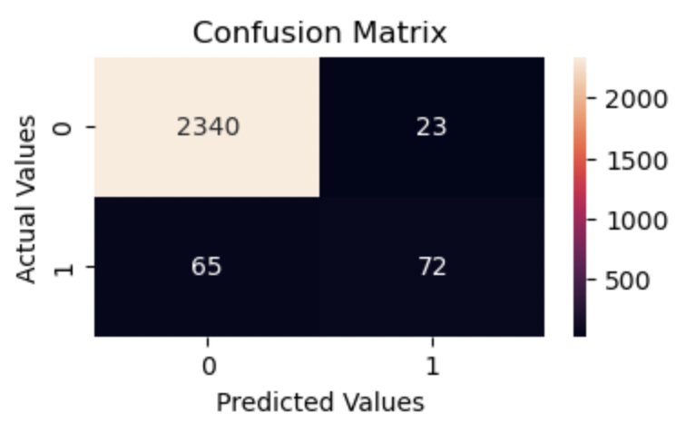
As highlighted before, the False Positives have drastically reduced from 483 to 23, and the True Positives have also reduced from 105 to 72, this is pretty decent. Additionally, the True Negatives have also improved considerably from 1,880 to 2,340. Generally, we can say that this classifier performed a bit better than the previous Logistic Regression model we built. You can also experiment with soft voting to see how that improves the classifier.

The Same Algorithm, Different Subsets of the Data

Here, we will be using the BaggingClassifier() method and the estimator(s) to be trained are Decision Trees.

from sklearn.ensemble import BaggingClassifier
from sklearn.tree import DecisionTreeClassifier

forest = BaggingClassifier(DecisionTreeClassifier(class_weight = "balanced"),
                           n_estimators = 500,
                           max_samples = 1000,
                           n_jobs = -1)

forest.fit(x_train, y_train)
y_pred = forest.predict(x_test)
compute_metrics(y_test, y_pred)

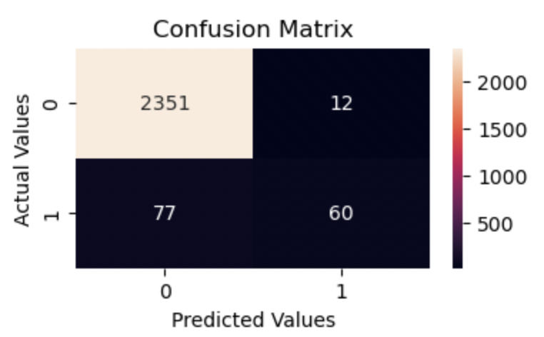
From the results above, the collection of decision trees performs decently on the data, not as well as the voting classifier, but far better than the Logistic Regression model we built earlier. The True Positives and True Negatives are close to the previous result. Let’s get more insight into what’s happening from the code.

500 decision tree classifiers are trained on the data with each taking a maximum number of 1,000 random samples. This means that each decision tree trains on a subset of the data, 1,000 samples to be precise. Additionally, I’m sure you noticed that this classifier is instantiated with the variable name forest. Aside from the catch that “many trees make a forest”, this is also a pointer to something else.

A collection of decision trees is a random forest classifier. And so, rather than creating the algorithm manually with the BaggingClassifier() method, we can simple use scikit-learn's RandomForestClassifier algorithm directly. Let's see if the results of the latter will be similar.

from sklearn.ensemble import RandomForestClassifier
rfc = RandomForestClassifier(class_weight = 'balanced')

rfc.fit(x_train, y_train)
y_pred = rfc.predict(x_test)
compute_metrics(y_test, y_pred)

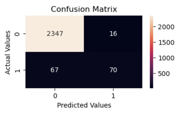
The algorithms perform similarly on the data. However, the are higher number of True Positives from the RandomForestClassifier algorithm, 70, compared to 60 by the BaggingClassifier(). This is possible because the RandomForestClassifier makes use of more parameters than what we specified in the BagginClassifier, making room for more dynamism and performance.

In Conclusion

In this article, we looked at the combination ensemble learning and class weight balancing as a method of dealing with class imbalance. From the results in the matrices indicated above, this combinatory method works better than training a single algorithm on imblanced data.

In the second part of this article, we will look into the boosting and stacking approaches to ensemble learning, how they are created and how they will perform.

Further Reading:

• A Comprehensive Guide to Ensemble Learning: What Exactly Do You Need to Know
• A Comprehensive Guide to Ensemble Learning (with Python codes)
• Ensemble methods: bagging, boosting, and stacking