Data science is a vast realm brimming with groundbreaking techniques designed to conquer intricate challenges. Enter the autoencoder, a game-changer that has ignited a revolution among machine learning, deep learning, and computer vision experts. With a wealth of data at our fingertips, autoencoders have sparked a wave of experimentation, propelling advancements in feature extraction, data augmentation, and beyond.

But what if you're new to this remarkable algorithm and its untapped potential? Fear not, for you've arrived at the perfect destination. Join us on an exhilarating journey as we demystify autoencoders, shedding light on their inner workings and unraveling their secrets.

Prepare for an enlightening adventure as we define the concept and dissect its structure. Once we've laid the groundwork, we'll explore the myriad applications of autoencoders, opening your eyes to their remarkable versatility. To top it off, we'll work through a concise tutorial on constructing your very own autoencoder.

Get ready to unleash the full potential of autoencoders—your gateway to the future of data science awaits!

Requirements

While there are attempts to simplify complex concepts for ease of comprehension, it is recommended that you have a basic grasp of the following to fully engage with the content:

1. Python, preferably, version 3.8.0 upward.

2. A deep learning framework of your choice, either Tensorflow or Pytorch

3. An understanding of Convolutional Neural Networks (CNN) and Deep Learning in general

It is also essential for you to have an IDE to practice with. There are tons of options to choose from here

With this out of the way, let's begin!

What is an Autoencoder?

An autoencoder is an algorithm used to regenerate and in some cases, manipulate various forms of data in a desired way. These could include, images, texts, videos, audio or what have you. These manipulations can be aimed at data denoising, augmentation, manipulation, and so on.

This algorithm is made up of two distinct parts which work together: an encoder and a decoder. The encoder changes the representation of the data from its original form to vectors, a form useful to the decoder and any other algorithm. The decoder’s job is the exact opposite. It works to transform the vectors into some output. (This could be the same image as the autoencoder received as input, a manipulated one, or an entirely different image).

Mathematically, we can represent these points as follows:

$$x → f(x) → \vec{V}$$

$$\vec{V} → f(x) → x$$

where:

• x is the input data

• f(x) is the encoder/ decoder as the case may be

• V is the representation of the data

Structure of an Autoencoder

An autoencoder is made up of an input layer and an output layer with different layers in between. These layers are shared between the encoder and decoder networks.

The input layer takes in a data observation (x). Usually, this layer has as many neurons as the number of features in the data being ingested. With little or no manipulations, the output of this layer serves as input to a hidden layer (L1), and so on. As the data proceeds through the encoding part of the algorithm, it gets compressed into smaller dimensions (with the help of a pooling layer), till it gets to the latent layer. Here, the final output of the encoder is projected as input for the decoding part of the algorithm.

The decoder takes the output from the latent layer and tries to expand it as the data proceeds through its own set of layers. This is because it aims to reconstruct the data back to its original form and size. columns in the data get repeated with the help of an up-sampling layer, till the data reaches the output layer.

A worthy point to note is how the neurons in an autoencoder's layer get smaller or larger as more layers are added. In some examples, the input layer can have N a number of neurons, determined by the number of input features and maybe a padding function. This number is usually halved as the layers progress, till the latent layer is reached. Proceeding from the latent layer, the number of neurons is doubled till the output layer is reached.

Think of it this way:

The Applications of Autoencoders

Autoencoders have various applications, here are a few notable ones:

1. Dimensionality reduction: As explained above, the encoder in an autoencoder, transforms input data into a smaller representation (n-dimensional vector). This makes it useful in reducing the dimensionality of data.

2. Data Denoising: Sometimes the data we work with (be it an image or audio) has some unwanted signals (noise) we want to get rid of. An autoencoder in this case can be used to generate a denoised version of the input data, by learning a cleaner representation of the data.

3. Recommendation Systems: Autoencoders are not recommenders themselves, but can be used in the process of recommending. The encoding part of the algorithm learns and produces vector representations of products in a customer’s purchasing history, as well as those in the inventory. Once this is completed, a Nearest Neighbours algorithm loops through the batch to get products that are similar to each other, and recommend these to the customer.

4. Anomaly Detection: Autoencoders are also useful for anomaly detection. The logic behind this is the reconstruction error (calculated by a loss function) which will be higher for images that a strange to an autoencoder, compared to images that are similar to what it is used to. For example, by training an autoencoder on the Fashion MNIST dataset, and then feeding it an image of a car for inference, the reconstruction error will be higher because there are no cars in the Fashion MNIST dataset and it is not used to seeing a car.

5. Information Retrieval: In information retrieval, we need the encoding part of the algorithm to compute representations of the input data (a query) as well as other objects in a database. A KNN or distance metrics like Euclidean distance or cosine similarities can then be used to compare and retrieve data objects close to the query.

Building an Autoencoder in Tensorflow

Building an autoencoder is surprisingly easy, we will be doing this with TensorFlow, and training it on the fashion MNIST dataset.

The fashion MNIST is one of the many datasets in Machine Learning used to develop and even benchmark algorithms. It consists of images of clothing and wears such as shoes, T-shirts, pullovers, trousers, etc. In terms of complexity, it is a bit more dynamic than the MNIST dataset which is made up of images of handwritten numbers of 0 through 9. The data contains 60,000 images for training, 10,000 images for testing, and a total of 9 unique target labels in all. Each image is a small square of size 28 28 1. This means, 28 in height and width and 1 in terms of depth (being grayscale images, there is only 1 color channel).

To build the autoencoder we don’t need the target labels, but rather than discard it, we can use them to label plots of fashion items.

Loading and Processing the Data

Open-source machine learning libraries like Scikit-learn and Tensorflow haveir own versions of the Fashion MNIST dataset. Since we will be using the latter to build our autoencoder, we will be loading the dataset this way:

(X_train_full, y_train_full), (X_test, y_test) = tf.keras.datasets.fashion_mnist.load_data()

The X_train_full will be split into train and validation sets, so it makes more sense to name it this way.

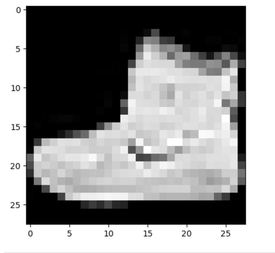
If you choose to preview the first image in the training data, you will observe some properties. Aside from the shape of the image, which has been explained previously, you will also see that the image is represented with numbers. These numbers are pixels ranging from 0 to 255. As the value of the pixel moves away from 0 or gets higher, the brighter the pixel becomes, the brightest being 255.

Let’s plot the first vector in the data to see what image we get. Although it is not so clear, this looks like a shoe.

Processing the data is also an easy step. Since we know that the pixel values are numbers between 0 and 255, we can normalize them. Normalizing numerical values improves the performance of Neural Networks as the gradients become more stable during training. If the gradients are stable, the model parameters get updated optimally, and we can reduce the error the model makes in reconstructing the images.

Normalizing is as easy as dividing the data by the maximum pixel value (255). This will give us values between 0 and 1.

X_train_full = X_train_full / 225.0

X_test = X_test / 225.0

Constructing the Autoencoder

The Encoder

1. An input Layer of 32 convolutional filters, 3 x 3 kernel size, a ReLU activation function, a padding layer, and an input shape of 28 x 28 x 1. The padding will of course ensure the size of the images becomes 32 x 32.

2. A max-pooling layer of size 2 x 2 to extract the high-level features of the images.

3. A Hidden convolutional layer of 16 filters, 3 x 3 kernel size, a ReLU activation function, and a padding layer.

4. Another Max pooling layer of size 2 x 2 to further summarise or extract the high-level features from the previous layer

5. A second hidden convolutional layer of 8 filters, 3 x 3 kernel size, a ReLU activation function, and a padding layer,

Another Max pooling layer of size 2 x 2 to further summarise or extract the high-level features from the previous layer. In the code pasted below, this will be named the encoded layer

The Decoder

As opposed to the encoder, we will be using up-sampling layers in the decoder, to increase the features extracted by the encoder. As mentioned previously, the job of the up-sampling layer is to repeat the columns and rows in the image representations such that the decoder’s output size is the same as the input image.

As such, the Decoder will be constructed in this manner

1. A Convolutional layer of 8 x 8 filters, 3 x 3 kernel size, a ReLU activation function, and padding

2. An Up Sampling layer of size 2 x 2 to increase the size of the image representations.

3. Another Convolutional Layer of 16 filters, with 3 x 3 kernel size, a ReLU activation function, and padding

4. Another Up Sampling layer of 2 x 2 to further increase the size of the image representations

5. A third Convolutional Layer of 16 filters, with 3 x 3 kernel size, a ReLU activation function, this time without paddareg (there is no use padding image representations of size 32 x 32 if the input size was already 32 x 32).

6. Another Up Sampling layer of 2 x 2 to further increase the size of the image representations

7. The last Convolutional Layer of 1 filter, with 3 x 3 kernel size, a Sigmoid activation function, with padding. This layer is usually called the decoded layer

The autoencoder is built with the Functional API in TensorFlow, which means we must concatenate the input layer with the decoded layer to complete the construction of the model. You can find the code for this step in the GitHub link attached at the end of this article. This doesn’t mean we can’t build a model with the Sequential API. The Functional API works best as the model can leverage the many connections between layers in our architecture for improved performance.

Compiling and Fitting the Model

As in every other case of deep learning with TensorFlow, you must compile the model. This is the only way by which you can tell the model what optimizer and loss function to use. In our case we will use the Stochastic Gradient Descent optimizer, to update the parameters of the model.

Once the compilation is completed without any errors, we get to the fun part which is fitting the autoencoder. Remember, our objective is to build an algorithm that can replicate the input image. To do this, we need to fit the model on the independent training features and evaluate its performance on a validation set.

The first thing we must do before training is to extract a validation set from the X_train_full dataset. We can easily do this with scikit-learn’s train_test_split() function. With this completed, we go ahead to fit the model, like so:

history = autoencoder_model.fit(X_train, X_train, epochs = 10, validation_data = (X_valid, X_valid))

You should see some logs detailing the number of times the model goes over the data (this is determined by the number of epochs set), the training and validation loss scores.

Instead of training the model on X, y samples and evaluating on the same as we do in classification and regression problems, we are fitting the model with X and X samples. This is in line with the objective of the task. If this was a classification problem, the aforestated will be preferred.

The model’s performance on the validation set, looks descent, having reduced from 0.3157 in the first epoch to 0.2715 in the last epoch. We also realize that there isn’t much overfitting going on, giving us the confidence that the model will be able to generalize effectively during inference.

You can derive the structure of the model with this code: autoencoder_model.summary().

Extracting the Encoder and Decoder

Now that we have trained the autoencoder, we can extract its parts for use separately and together. The encoder will help us encode Fashion MNIST-related images into n-dimensional vectors, while the decoder can help us transform such vectors back into images.

encoder = tf.keras.models.Sequential()

decoder = tf.keras.models.Sequential()

for layer in autoencoder_model.layers[:8]:

encoder.add(layer)

for layer in autoencoder_model.layers[8:]:

decoder.add(layer)

Extraction is done by creating empty sequential models for both the encoder and decoder, and then iteratively attaching each layer to their respective model objects.

We can then test these on unseen images

Regenerating Input Images

Applying the aforementioned models is possible with the predict() method, which is used in this way:

encoder_predictions = encoder.predict(sample)

decoder_predictions = decoder.predict(encoder_predictions)

For reference, these are the images we want to regenerate:

Once we get the encoded representations of these images, we pass them through the decoder as indicated above, and then we get the input images back:

The images are noticeably blurry, but visually, we can tell that they are regenerated versions of the input images. We can also tell with cosine similarities. We simply flatten the actual and predicted vectors and try to calculate how close they are to each other. The higher the value we get in return, the similar they are, and vice versa. We can do this with this bit of code. Here we will just take up the first image in the predicted and regenerated images.

from scipy.spatial.distance import cosine

1 - cosine(decoder_predictions[0].flatten(), sample[0].flatten())

We subtract the output from one (1) because Scipy’s cosine method calculates the distance and not the similarities. The distance, therefore, needs to be subtracted from 1 to get how similar the input vectors are.

The above computation gives us 0.9236, giving us the impression that the two images are similar.

Conclusion

In this article, we discussed the fundamentals of autoencoders, their structures, and parts. We also delved into practical implementation steps, by training a model with the Fashion MNIST dataset, evaluating it on a validation set, and testing out its regeneration capabilities on unseen data.

Autoencoders have more potential beyond image reconstruction and are useful for feature extraction, data augmentation and manipulation, recommender systems, and much more.

You can go beyond the purview of this article, to explore these capabilities, and put them to good use in your day-to-day job. Please let me know what you find :)