


Photo by Planet Volumes on Unsplash
An Implementation of the Nearest Neighbours Algorithm from Scratch in Python


I recently came across an intriguing fact about doppelgangers. People who look alike but are not related tend to behave similarly and have similar genetic profiles. You can read more about this fascinating fact here. This means that anyone who resembles you but is not related to you is likely to exhibit behaviours similar to yours.
This notion of similarity is also present in data science and is used in various techniques such as similarity learning, similarity search, and even algorithms like Nearest Neighbours.
In this article, I will be discussing the Nearest Neighbours algorithm, and also implementing it from scratch in Python. I will also highlight aspects of Machine Learning where this algorithm can be applied.
You can follow through even if you don’t have technical depth or background on the topic at hand, I have tried to make the topic simple to grasp, by defining terms and adding links to easy-to-understand articles that can dive deeper where I just scratched the surface.
Definition of Frequently Used Terms
Before jumping deep into this conversation, I like to clarify a few terms.
Algorithm: An algorithm is a system of rules and logic created to achieve a certain outcome.
Distance: In this context, distance is a measure of how different vectors and/ or other representations of data are. This measure gives us a sense of how similar or dissimilar they are. Common distance metrics in data science are cosine distance (also called cosine similarities), Euclidean distance, manhattan or cityblock distance, etc.
Classification: A technique in Machine Learning, in which data observations are categorized under pre-defined “classes”. These classes are discrete variables which represent categories.
Regression: A technique in Machine Learning, in which a target variable, consisting of continuous values is estimated. These values are termed continuous because they measure certain things, for example, the selling price of a house, the average height of toddlers by gender, etc.
The Nearest Neighbours Algorithm
Nearest neighbours is an algorithm that has applications in different use cases including search, classification, regression, etc. It is built on the principle that objects in an n-dimensional space that are similar are closer than objects that are not. In classification, a variant of this algorithm is the K-Nearest Neighbours algorithm which simply predicts the most frequent class it has observed during training for a new and similar data point. In regression, it averages out the target variable, all of this dependent on the number of (K) instances it is configured to consider.
The origins of this algorithm are traced to the work of Evelyn Fix and Joseph Lawson Hodges Jr. in their work titled Discriminatory Analysis - Nonparametric Discrimination: Consistency Properties. In their research, Fix and Hodges demonstrated that it is possible with Euclidean distance to compare different samples with each other and identify K instances that are closer together. Some years later, Thomas Cover adapted the Nearest Neighbours algorithm to a classification task, submitting that a new sample/ instance of data can be classified into the same class as its nearest data sample.
This algorithm is often described as a lazy learner, a type of algorithm that does not learn any patterns from training data. In most cases, it simply stores or retains some information about the data. When fed new data for predictions, the lazy learner runs through training data and generates some inferences based on the information captured therein.
To its advantage, the Nearest Neighbours algorithm is known for its simplicity, along with its performance on different tasks. In a study that coupled the Nearest Neighbours algorithm with Parallel computing, researchers Yijie Dang, Nan Jiang, Hao Hu, Zhuoxiao Ji and Wenyin Zhang demonstrated that this algorithm can attain 83% classification accuracy on image classification tasks.
How the Algorithm Works
The inner workings of the Nearest Neighbour Algorithm in most cases depend on the type of problem it is being adapted to. Notwithstanding, the algorithm has the following steps
Store the training or learning dataset;
Upon seeing a new data point to be extrapolated upon, run through the stored data, computing a distance metric between each observation and the new data point;
Retrieve the most similar instances according to the distance metric computed - The lesser the distance the more similar the training instance is to the new data point:
In a classification case, compute the Mode of classes of the training instances retrieved
In a regression case, compute the average (mean) of the target variables for the training instances retrieved.
In an information retrieval scenario, simply return the training instances.
For better understanding, we have this written in Python code:
import numpy as np

def euclidean_distance(X_old, X_new):
    return np.sqrt(np.sum((X_old - X_new) **2, axis = 1))

def manhattan_distance(X_old, X_new):
    return np.sum(np.abs(X_test[0] - X_train), axis = 1)


class NearestNeighbours():
    def __init__(self, K, distance_func, adaptation):
        self.K = K
        self.distance_func = distance_func
        self.adaptation = adaptation

    def _fetch_top_K(self, X_old, X_new):
        distances = self.distance_func(X_new, X_old)
        top_K_indices = np.argsort(distances)
        return top_K_indices[:self.K], distances[top_K_indices]

    def store_train_set(self, X, y):
        self.X = X
        self.y = y
        return self.__class__.__name__

    def retrieve(self, X_new):
        top_K_indices, distances = self._fetch_top_K(self.X, X_new)
        return self.X[top_K_indices]

    def _predict_classification(self, X_new):
        top_k_indices = self._fetch_top_K(self.X, X_new)
        most_frequent_target = Counter(
                           Self.y[top_k_indices]
        ).most_common(1)[0][0]
        return most_frequent_target

    def _predict_regression(self, X_new):
        top_k_indices = self._fetch_top_K(self.X, X_new)
        average_target = np.mean(self.y[top_k_indices])
        return average_target

    def predict(self, X_new):
        if self.adaptation == 'classification':
            return self._predict_classification(X_new)
        if self.adaptation == 'regression':
            return self._predict_regression(X_new)
Here we have four (4) code blocks, the first imports the NumPy library which is used at different points in the algorithm, and the second and third blocks are the distance metrics which we will talk about subsequently. The fourth block of code is a class object which encapsulates the Nearest Neighbours algorithm as described in the previous sections.
Now in detail, I will describe what these functions and class methods do:
euclidean_distance: Euclidean distance is a distance metric that can be used to calculate the length between two (2) points.
Let’s assume that there are two points A and B. The Square root of the sum of the squared differences between A and B will give us a measure of how B is distant from A. Mathematically we can describe Euclidean distance as: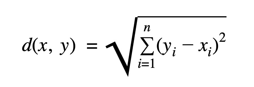
manhattan_distance: Manhattan distance is also called cityblock distance, as opposed to its counterpart, it is the sum of the absolute difference between two points. Mathematically, it is defined as:
_store_train_set: This method in the algorithm is synonymous with the fit() method in scikit-learn’s implementation of the algorithm, its task is to store the training data in the algorithm. It returns the name of the algorithm, as a confirmation that it has stored the training set.
_fetch_top_K: As the name suggests, it fetches the most similar observations to the newly observed sample, from the training set. In doing so, it makes use of the distance function specified. It returns two objects, the first an array of integers which represents the closest to the Kth element, where K is the number of neighbours to be considered; and the distances.
retrieve: The retrieve function is used in a search and information retrieval situation, if we wish to search for documents or objects that provide answers to a query, we can use the retrieve function.
predict: This is used in a classification or regression case and works well with tabular data. If we wish to use the algorithm for a classification task, it returns for a new observation, the most frequent class observed among that observation’s nearest neighbours. In a regression task, it simply computes an average of the target labels observed in that observation’s nearest neighbours.
Demonstration
Now that the algorithm has been explained and implemented with the Python programming language, I will demonstrate the uses of this algorithm in Search, Classification and Regression.
Search and Retrieval
In this demonstration of the Nearest Neighbours algorithm, I will show how it can be used to retrieve items in the training set, based on their similarity to the unseen observation. To give a sense of performance, I will also make use of scikit learn’s implementation of the algorithm as well and compare the results to check for a deviation.
Our Custom Implementation of Nearest Neighbours
X_search_train = np.random.randint(0, 100, size = (10, 10))
X_search_test = np.random.randint(0, 100, size = (1, 10))
search_model = NearestNeighbours(
    K = 5,
    distance_func = euclidean_distance,
    adaptation = 'search'
)
search_model.store_train_set(X_search_train, y = None)
search_model.retrieve(X_search_test)


## OUTPUT:


(array([[30, 41, 51, 92, 28, 60, 15, 51, 22, 65],
        [46, 62, 92, 32,  2, 83, 91, 75, 55, 91],
        [42,  2, 83, 82, 65,  6, 55, 71, 37, 52],
        [83, 15, 83, 80, 62,  9, 25, 70, 22, 75],
        [90, 63, 65, 53, 23, 71, 28, 41, 60, 41]]),
 array([ 80.14362108,  98.0663041 , 119.36079758, 125.51493935,
        126.1308844 ]))
Scikit-Learn’s Implementation of Nearest Neighbours
from sklearn.neighbors import NearestNeighbors

nbrs = NearestNeighbors(
        n_neighbors=5,
        algorithm='ball_tree'
).fit(X_search_train)
distances, indices = nbrs.kneighbors([X_search_test[0]])
X_search_train[indices], distances

## OUTPUT:


(array([[[30, 41, 51, 92, 28, 60, 15, 51, 22, 65],
         [46, 62, 92, 32,  2, 83, 91, 75, 55, 91],
         [42,  2, 83, 82, 65,  6, 55, 71, 37, 52],
         [83, 15, 83, 80, 62,  9, 25, 70, 22, 75],
         [90, 63, 65, 53, 23, 71, 28, 41, 60, 41]]]),
 array([[ 80.14362108,  98.0663041 , 119.36079758, 125.51493935,
         126.1308844 ]]))
Classification
As done for the Search and Retrieval, I will also do for classification, by generating synthetic data with scikit-learn’s make classification method.
X, y = make_classification()

from sklearn.model_selection import train_test_split

X_train, X_test, y_train, y_test = train_test_split(X, y, stratify = y)

model = NearestNeighbours(
K = 5,
distance_func = euclidean_distance,
adaptation = 'classification
')

model.store_train_set(X_train, y_train)
model.predict(X_test[0])

Actual target value: 0

## OUTPUT:

0
With scikit-learn’s adaptation of the Nearest Neighbours algorithm to classification (KNearestNeighbors), we see the same output
from sklearn.neighbors import KNeighborsClassifier

sklearn_model = KNeighborsClassifier(n_neighbors = 5)
sklearn_model.fit(X_train, y_train)
sklearn_model.predict([X_test[0]])

Actual target value: 0

## OUTPUT:

array([0])
Regression
X, y = make_regression()

from sklearn.model_selection import train_test_split

X_train, X_test, y_train, y_test = train_test_split(X, y)

model = NearestNeighbours(
K = 5,
distance_func = euclidean_distance,
adaptation = 'regression'
)

model.store_train_set(X_train, y_train)

model.predict(X_test[0])

## Actual target value: 285.3488884348154

## OUTPUT:

139.42246741707405
Scikit-learn’s implementation (KNearestNeighbors)
from sklearn.neighbors import KNeighborsRegressor
sklearn_model = KNeighborsRegressor(n_neighbors = 5)
sklearn_model.fit(X_train, y_train)
sklearn_model.predict([X_test[0]])


## Actual target value: 285.3488884348154


## OUTPUT:

array([139.42246742])
Limitations of the Nearest Neighbours Algorithm
While its simplicity and performance is a plus, it is not without limitations. There are two major limitations I like to discuss.
Computationally expensive and requires high storage space: The Nearest Neighbours algorithm needs to store the training set to be able to make inferences on unseen data. Depending on the size of the data, this might require high storage space. Additionally, the algorithm needs to walk through the training set each time it is fed an unseen data observation.
Considers no information about the training set: Unlike linear models, Tree-based models, etc, the Nearest Neighbours algorithm pays no attention to the underlying distribution of the training data and so does not learn any patterns. When the datasets (train and test) are without noise or outliers, this is not a limitation. When the converse is the case, however, the performance of the algorithm is affected.
Like every other algorithm in the world of Data Science, the Nearest Neighbours algorithm has its strengths and weaknesses. Notwithstanding, it is a fundamental algorithm that can be used in use cases that require small to medium-sized data sets
With this, it is likely that you now have an understanding of how this algorithm works and the areas in which it can be applied.