Heart Disease otherwise called Cardiovascular disease (CVD) is an umbrella term for a number of conditions that affect the heart. You can find an extensive list of conditions that qualify as heart disease here. For simplicity and ease of understanding, I will be treating "heart disease" as a singular unit (i.e. one disease) in this article.

CVD is the number one cause of death in the world. The Global Burden of Disease records that out of the 56 million people who died in 2017, 18.56 million were killed by Cardiovascular disease, that’s 33.14%.

It is also the leading cause of death in the United States.The CDC estimates that every 36 seconds, an American dies from heart disease. Similarly, this disease also claims preponderance among the causes of death in Nigeria.

Accordingly, Ischemic heart disease is ranked as the sixth leading cause of death in Africa's most populous nation. Statista estimates that in 2019, 5.18% of all deaths resulted from this condition.

With this in mind, combatting heart disease as it is discovered in patients might not be of great help in reducing its spate of killings and, may seem a bit like a rat race anywhere in the world. This is because heart disease is faster at occurring (and killing) than we are at stopping it from doing so. Hence, we need to be "one step ahead" of the disease.

What if we could know those that are likely to develop this condition, even before they actually do?

It’s been proven in a study published in PLoS ONE that Machine Learning can reduce the occurrence of heart disease by identifying people with a likelihood of developing the ailment.

Therefore, an effective approach to combatting heart disease will have an ML model at its core, to identify those that may develop the ailment in the future.

With this sample data from Kaggle, I will be demonstrating in this article how such a model can be built. You can also find the code I used for this task in this repository.

Prerequisites To follow this tutorial

To follow this piece, you might need:

• An understanding of Machine Learning particularly binary classification
• Basic to intermediate understanding of the sklearn library
• Intermediate Python skills, and knowledge of Pandas library and its methods

If you do not have the aforementioned prerequisite knowledge and you’ll like to go on, please feel free, I will do my best to explain technical concepts along the way. I have also indicated links to articles that can help your understanding where my explanations may not suffice.

Building the Model

First things first; a model (a machine learning algorithm trained on data) represents the relationship between an independent and dependent variable(s). And yes, I am implying that a model and an ML algorithm are not the same things. That distinction is spelled out here.

This means that; when the dependent variable is absent or needs to be identified, a model can help us infer to a certain degree, what that variable might be. It can do this, by identifying inherent patterns in the independent variable(s).

In building this model (heart disease predictor), I followed these steps:

1. Data Collection
2. Data Cleaning and Processing
3. Exploring the Data
4. Preparing the Data for Modeling
5. Choosing the “right” Model
6. Predicting Likelihood

Data Collection

Collecting data is the foundational step in any Machine Learning project. As mentioned previously, I collected the data from Kaggle with the help of these API commands.

# download zipped file from kaggle with kaggle API command
!kaggle datasets download --force 'kamilpytlak/personal-key-indicators-of-heart-disease'

# unzip the file to access the dataset. 
!unzip personal-key-indicators-of-heart-disease.zip

The dataset was curated by the CDC (Centre for Disease Control) as part of its Behavioral Risk Factor Surveillance System (BRFSS) and collected from a total of 401,958 people. Questions such as "Do you have serious difficulty walking or climbing stairs?" or "Have you smoked at least 100 cigarettes in your entire life?” were answered by respondents. This survey process resulted in a dataset consisting of 319,795 observations by 18 columns.

To help you understand the data more effectively, I have classified the columns into themes.

let's dive deep into what the data contains

Lifestyle Habits:

• AlcoholDrinking (Boolean): Yes if the patient drinks alcohol and No if the patient does not
• Smoking (Boolean): Yes if the patient smokes and No if the patient does not
• SleepTime (Float): The time of the day the patient goes to bed
• physical activity (Boolean): If the patient engages in physical activities or not, yes if the patient does, no if they don’t
• PhysicalHealth (Float): Number of days in the last 30 days the patient has worried about their physical health
• MentalHealth (Float):Number of days in the last 30 days the patient has worried about their mental health
  

General Health Information:

• GenHealth (Object): The patient's perspective of their health. Terms such as Very good, Good, Excellent, Fair, Poor measure these perspectives.
• BMI (Float): Body Mass Index of the patient, a measure of body fat based on height and weight

Demographic Information:

• AgeCategory (Object): The age group of the patient. Age groups in the data include: 18-24, 25-29, 30-34, 35-39, 40-44, 45-49, 50-54, 55-59, 60-64, 65-69, 70-74, 75-79, 80 or older
• Sex (Object): The gender of the patient, either male or female
• Race (Object): Race of the patient. The patient can be from any of the following races: American Indian/Alaskan Native, Asian, Black, Hispanic, Other, White

Health Conditions:

• Diabetic (Object): Indicates if the patient is diabetic, prediabetic, had diabetes during pregnancy, or not diabetic
• DiffWalking (Boolean): Indicates if the patient has difficulty walking or not
• KidneyDisease (Boolean): Indicates if the patient has kidney disease or not
• SkinCancer (Boolean): Indicates if the patient has skin cancer or not.
• Asthma (Boolean): Indicates if the patient has Asthma or not.
• Stroke (Boolean): If the patient has a stroke or not.
• HeartDisease (Dependent Variable) (Boolean): The variable we are trying to predict. If the patient has heart disease or not.

I'm sure you are wondering why the variable we are trying to predict is already in the data, It's pretty simple. In Machine Learning, algorithms are taught by examples. These features and the values we are trying to predict are examples that any chosen algorithm will learn from. By doing so, the trained model will repeat what it has learned from these examples on data it has not been exposed to.

Data Cleaning and Processing

It is safe to assume that data will be messy in most scenarios. This makes it a good idea to check for missing values, outliers, duplicates with case distinctions (e.g. heart, Heart). Thankfully, in this case, there wasn’t anything like the issues mentioned above. But should you run into missing data, this article will help you out. You can also take a look at this article to guide you in data cleaning.

I generated a statistical summary of the numerical attributes in the data with Pandas’ .describe() method. This gave me a sense of the central tendency, dispersion and distribution of these columns.

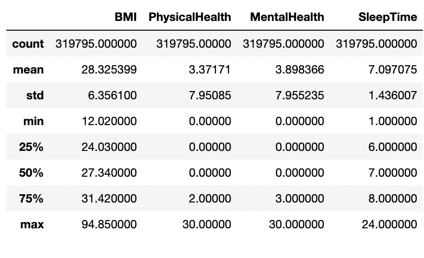
The minimum and maximum levels as seen in the image fall outside of the majority of the data which are within the 25th percentile and 75th percentile. Put differently, they do not follow the predominant patterns in the columns and as such, they can be considered as outliers.

For example, a BMI level of 94.65kg/m² is was above the 75th percentile in that column. In real-life scenarios, such a BMI level is almost impossible to have and may have only gotten into the data as a result of faulty imputation. The maximums of other numerical attributes can be ignored since an individual can worry about their health (mental or physical) for 30 days and go to bed at 24:00 (00:00 or midnight).

Rows with strange BMI measurements were identified with the Interquartile Range (IQR) (The difference between the third upper quartile and first lower quartile) and were then dropped from the data. The resulting dataset had 309,399 observations.

These numerical features are continuous, that is, there are large number of variables between the lowest (minimum) and highest (maximum) points. Visualizing these might be clumsy and pose a problem for human comprehension.

For this reason, I categorized these values into bins, this process is known as discretization. The numerical attributes were discretized as follows (please refer to these to guide you in reading the following information < = less than, > = greater than, ≤ = less than or equal to, ≥ = greater than or equal to):

BMI:

1. ≤18, Underweight
2. > 18 and ≤ 24, Normal
3. > 24 and ≤ 29, overweight
4. > 29 and ≤ 39, obese
5. > 39, extremely obese

MentalHealth and PhysicalHealth

1. ≤ 5, rarely concerned
2. > 5 and ≤ 15, often concerned
3. > 15, almost almost always concerned

SleepTime

1. ≤ 6, 00:00am - 06:00am
2. > 6 and ≤ 12, 06:00am - 12:00am
3. > 12 and ≤ 18, 12:00pm - 18:00pm
4. > 18 and ≤ 24, 18:00pm - 00:00pm

Exploring the Data

For this task, I conducted univariate and multivariate analysis. Univariate analysis is a type of analysis that focuses on one variable, while multivariate analysis involves more than two variables.

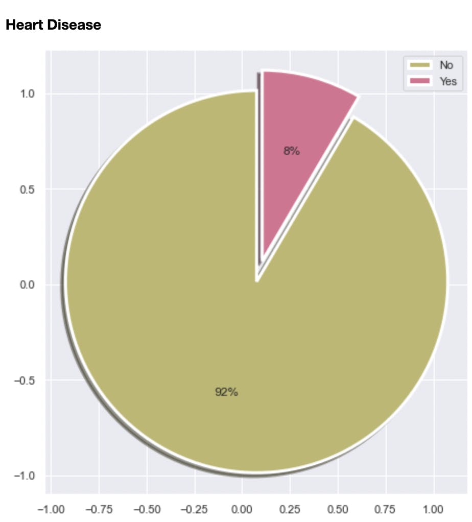
Among other things, the analysis helped me discover the class imbalance in the dataset. 92% of the data was labeled as “No” signifying not having heart disease and 8% was labeled as Yes. I will touch more on this in subsequent sections

It also helped identify some of the factors that increase the risk of heart disease. Some of these are:

• Going to bed late (between midnight and 12 noon)
• Smoking
• Being overweight or obese (Having BMI of 25 kg/m² and above)
• Being of age 65 or older
• Being male, (From the EDA, males are more likely to develop heart disease than females).
  

Please note that these insights are from a simulated observation. Contact your doctor on factors that can increase the likelihood of developing heart disease.

Preparing the Data for Modeling

After exploring the data, I dropped the numerical attributes in the data, since they had already been discretized to form new columns.

I also transformed the data into the required structure and representation, suitable for Machine Learning Algorithms, this is called preprocessing. Since all the columns in the data consisted of either boolean or object type values, the only preprocessing step needed here was encoding.

Encoding is simply the process of transforming categorical variables into numbers, for fitting into a Machine Learning algorithm. ML algorithms do not work well with strings. On the other hand, they are able to interpret numbers comfortably. For this reason, I encoded the strings with numbers.

Primarily, there are two types of encodings: One Hot Encoding and Ordinal Encoding. To understand how they work, you need to know the types of categorical variables there are.

Nominal and ordinal variables are the basic types of categorical variables that can be available in any given situation. While nominal variables do not contain any inherent order in them, Ordinal variables do. An example of a set of nominal variables is the Names of countries in the world. Except they are ranked based on a form of measurement like GDP, etc, there is no inherent order. Ordinal variables on the other hand include things such as strongly disagree, disagree, neutral, agree, and strongly agree. Here there is an order among the variables.

Ordinal variables are ordinally encoded to preserve the order and relationship between the variables, while nominal variables are one hot encoding. You can read this article to gain a better understanding

For this task, three types of encoders were used. These include label encoder, ordinal encoder and one hot encoder all created and managed by the scikit-learn library. Ordinal Encoder and One Hot Encoder were used for the independent categorical variables in the data while the dependent variable “HeartDisease” was encoded with the Label Encoder

See below for code snippets of how I used these encoders

one_hot_encoder = OneHotEncoder(handle_unknown = 'ignore')
ordinal_encoder = OrdinalEncoder()
LabelEncoder = LabelEncoder()

#identifying nominal and ordinal columns
nominal_columns = ['Sex', 'Race']
ordinal_columns = ['Smoking','AlcoholDrinking','AgeCategory','Stroke',
'DiffWalking','PhysicalActivity','GenHealth','Asthma','KidneyDisease',
'SkinCancer','weight_status_by_bmi','physical_health_status', 'mental_health_status','sleep_time_bins']

#one hot encoding nominal columns
one_hot_encoder.fit(x[nominal_columns])
ohe_columns = one_hot_encoder.transform(x[nominal_columns]).toarray()
ohe_columns = pd.DataFrame(ohe_columns, columns = one_hot_encoder.get_feature_names_out())

#encoding ordinal columns
ordinal_encoder.fit(x[ordinal_columns])
oe_columns = pd.DataFrame(ordinal_encoder.transform(x[ordinal_columns]), columns = ordinal_encoder.feature_names_in_)
oe_columns.head()


#label encoding y variables
LabelEncoder.fit(y)
y_transformed = LabelEncoder.transform(y)

#merging preprocessing results for independent variables
x_transformed = pd.concat([ohe_columns, oe_columns], axis = 1)

As previously mentioned, the EDA revealed the inherent class imbalance in the data (See Data Exploration) among other things. I resolved this by oversampling the minority class which in this case is “Yes” and undersampling the majority class which is “No”.

The danger of training an algorithm with unbalanced data is that it leads to poor predictive performance, where the model will rarely be able to predict the minority class correctly. This is problematic, especially for something as critical as heart disease.

To balance out the data I used the imblearn library this way:

from imblearn.pipeline import Pipeline
from imblearn.over_sampling import RandomOverSampler
from imblearn.under_sampling import RandomUnderSampler

# imblearn oversampling and undersampling to balance classes
over = RandomOverSampler(sampling_strategy= 'minority')
under = RandomUnderSampler(sampling_strategy= 'majority')
steps = [('o', over), ('u', under)]
class_balancer = Pipeline(steps=steps)


x_resampled, y_resampled = class_balancer.fit_resample(x_transformed, y_transformed)

Choosing the “right” model

Once class imbalance was resolved, I set about choosing the right model.

Selecting a model in Machine Learning is a scientific process that can among other things involve comparing different algorithms together based on their performance on the data. Performance is measured by how well the algorithms can identify hidden patterns and use that knowledge to predict outcomes for unseen data.

This implies that more than one algorithm will be trained and evaluated on a hold-out-set derived from the preprocessed data. The one that performs best based on the metrics is chosen.

Below are the lines of code that helped me achieve this:

# classifiers
gbc_clf = GradientBoostingClassifier(random_state = 42)
rfc_clf = RandomForestClassifier(random_state = 42)
log_reg = LogisticRegression(solver = 'liblinear', random_state = 42)
dt_clf = DecisionTreeClassifier(random_state = 42)


# splitting the data into train and test for evaluation
x_train, x_test, y_train, y_test = train_test_split(x_resampled, y_resampled, 
                                                   test_size = 0.2, stratify = y_resampled)

# computing precision, recall, train and test score and plot confusion matrix 
def compute_metrics(model, x_train, x_test, y_train, y_test, y_pred): 
    print('training_score:', model.score(x_train, y_train))
    print('testing_score:', model.score(x_test, y_test))
    print('difference between train and test score:', model.score(x_train, y_train) - model.score(x_test, y_test))
    print('precision_score:', precision_score(y_test, y_pred))
    print('recall_score:', recall_score(y_test, y_pred))
    cm = pd.DataFrame(confusion_matrix(y_test, y_pred))
    plt.figure(figsize=(8, 6))
    sns.heatmap(cm, annot=True, fmt='g')

    plt.title('Confusion Matrix')
    plt.ylabel('Actual Values')
    plt.xlabel('Predicted Values')
    plt.show()


for clf in [rfc_clf, gbc_clf, log_reg, dt_clf]:
    algorithm_name = clf.__class__.__name__
    display(Markdown('#### {} based model'.format(algorithm_name)))
    clf.fit(x_train, x_test)
    y_pred = clf.predict(x_test)
    compute_metrics(clf, x_train, x_test, y_train, y_test, y_pred)

Results of the Benchmarking Process

The following shows the performance of each model on the test set after training.

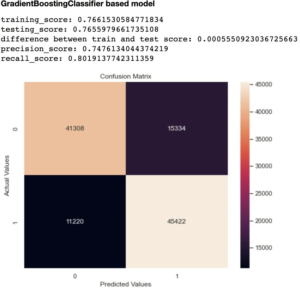
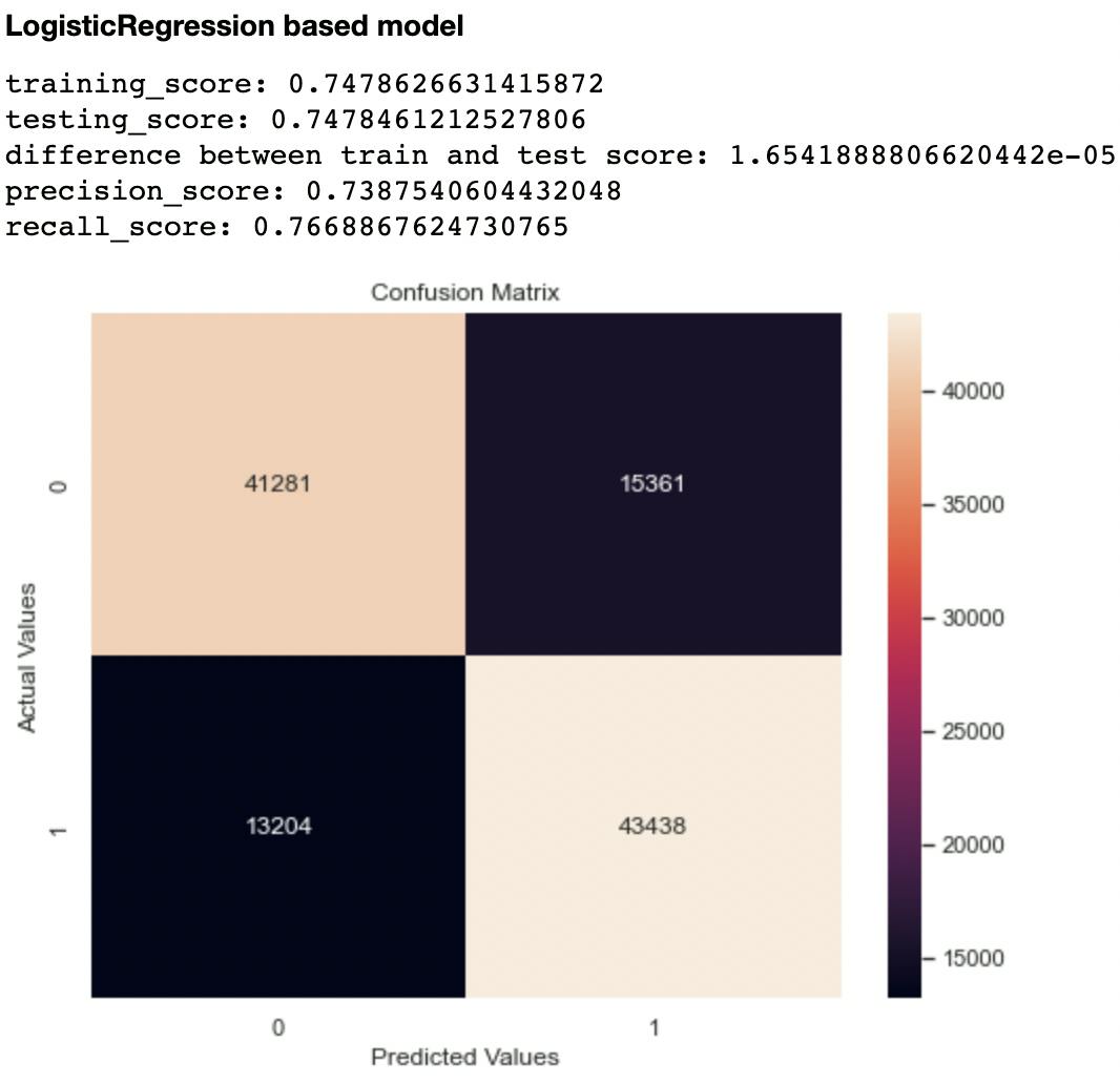
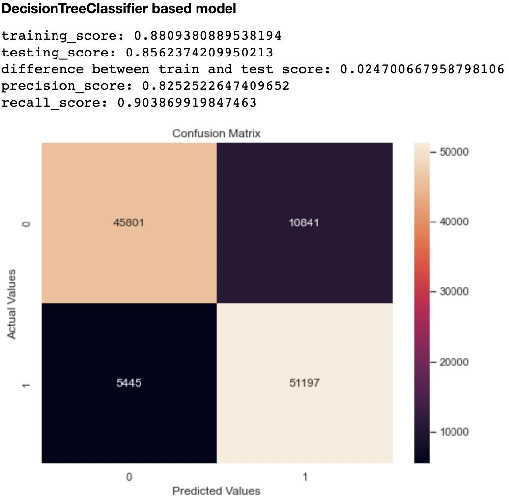
Out of the metrics generated for each model, I focused on recall and confusion matrix as the two evaluation metrics to compare the models. This is because recall (sensitivity or True Positive Rate) tells us how well a model can identify True Positives. It is calculated with this formula:

Recall_score = True Positive/ (True Positive + False Negative)

Imagine a scenario where a model predicts that an individual is not likely to develop heart disease, whereas this is a False Negative. That individual automatically misses out on preventive care and the end results can be catastrophic! Hence, choosing the right metric helps us not only evaluate or model but also optimize appropriately.

The second metric I considered was the confusion matrix, particularly the False Negatives and False Positives. A model that has high levels of these indices is likely to mislead health experts.

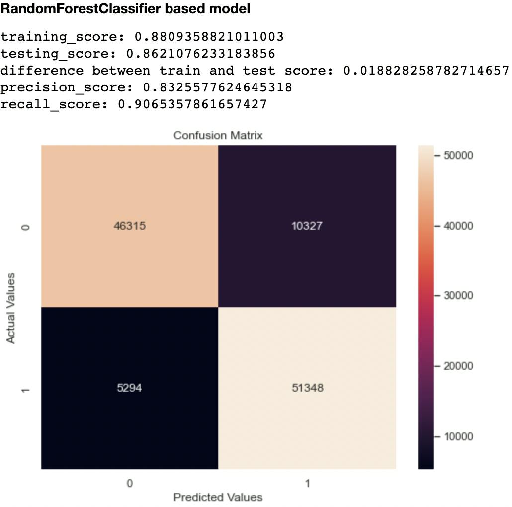
Out of all the classifiers trained, the Random Forest Classifier had the highest recall score at 0.906 and lowest False Negatives and Positives of 10,327 and 5,294 respectively. The closest performing model was the Decision Tree Classifier with a recall score of 0.903 and False Negatives and Positives of 10,841 and 5,445 respectively.

Can the Chosen Model Confirm Some Observations From the EDA?

Now that we have a model, we need to know what features inform its predictions, this is called feature importance. These features can be taken as indicators or factors that contribute to the development of heart disease and, can in a way, help confirm the observations of the EDA.

Here is a Horizontal Bar Chart that ranks features according to their levels of importance in the model’s predictions.

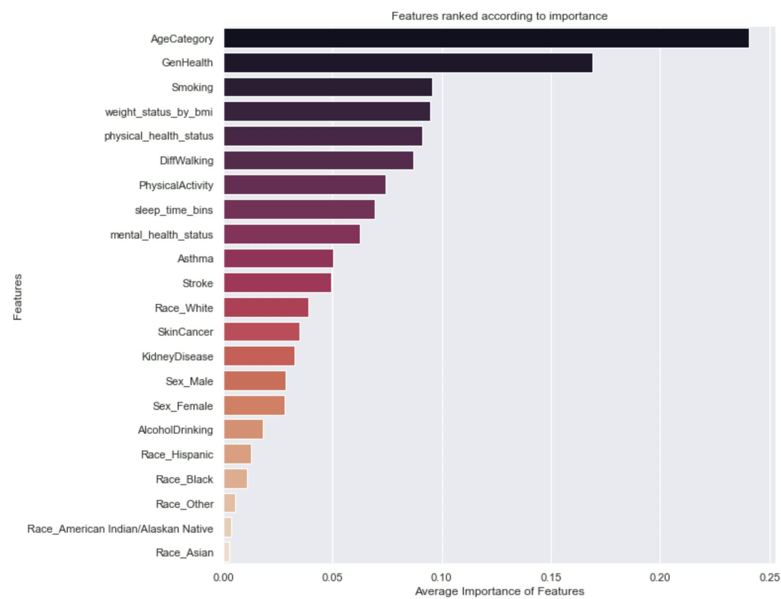
Interestingly, the model’s decisions are heavily influenced by Age, Perspective of general health and wellbeing, smoking habits, weight as indicated by BMI, and so on. Some of these features were already identified as risk factors in the EDA.

Predicting Likelihood

For the model to be useful, it shouldn’t only predict the discrete outcomes correctly (as measured by the metrics above) but predict the likelihood of developing heart disease, and correctly at that too, This speaks to probability. Generating probabilities for each prediction of the model helps us identify likelihood. As so for each “Yes” or “No” prediction made by the model, I generated a probability prediction. This was done with the predict_proba() function.

Applying these probabilities, we simply just need to identify people that are “more” likely to develop heart disease, depending on the set threshold. Someone with a probability score of 0.8 indicates a significant likelihood of developing the condition. Health centers can then be guided on how and whom to channel preventive care.

In Closing...

I followed these steps to build a model to predict likelihoods of developing heart disease, but they are not “cast in stone” (permanently fixed procedures). Changes can be made to these methods to improve predictive performance. Some of these include:

1. Normalizing numerical attributes as opposed to discretizing and ordinally encoding them
2. Making use of deep learning libraries like PyTorch and Tensorflow to build the model as opposed to sklearn.

I’m enthusiastic about solutions that use Machine Learning to improve quality of life, and I am willing to discuss this and other ideas you might have. You can reach me through my mail: seyiogunnowo@gmail.com, LinkedIn, or Twitter.