Machine Learning or ML is a type of Artificial intelligence that enables self learning from data and applies that learning without the need for human interventions. As a broad field, ML is divided into two major parts:

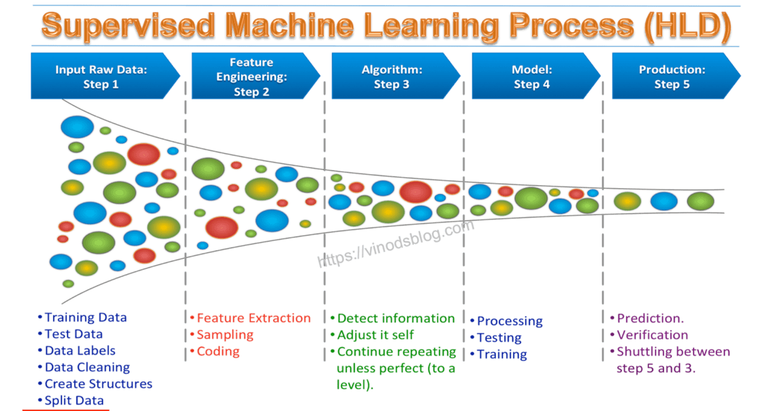
• Supervised learning: This is simply the process of training a machine or computer to identify patterns from labeled data. It aims to solve two kinds of problems:
  • Classification problems: This deals with predicting discrete values i.e. 0s and 1s, where 1=Yes, 0=No
  • Regression problems: This deals with predicting continuous values such as 0.11, 0.22, 0.33.
• Unsupervised learning: This is simply the process of drawing inferences and patterns from unlabeled data.

The focus of this tutorial will be on Supervised Learning to solve classification problems. I have highlighted below a project I have worked on to further buttress this.

Prerequisites to follow along with this tutorial

• Python
• Pandas
• matplotlib.pyplot
• scikit-learn
• OneHotEncoding

The Project: Predicting Consumer Behavior to Promo Sales

Case Scenario:

ABC enterprise specializes in the production and sales of cars. Recently, the company released an upgrade to the Series T, but executives were curious as to how many people will take advantage of this new promo.

Task:

Predict how many people will follow through with the just released promo based on past data

Solution:

Step 1: Data Collection

Data collection is the process of retrieving raw data concerning a previously well defined problem statement. In this case, the problem statement formed the foundation of the task above. Hence, the data collected was arranged in a tabular format with Location and other details including amounts customers had spent previously. The data is stored in a file called customer_data.csv

Step 2: Importing tools

import pandas as pd
from sklearn.linear_model import LogisticRegression
from sklearn.model_selection import train_test_split
from sklearn.preprocessing import MinMaxScaler
import matplotlib.pyplot as plt
data=pd.read_csv(customer_data.csv)
model=LogisticRegression(solver='liblinear', random_state=0)
scaler=MinMaxScaler()

logistic regression would be used to predict discrete values. MinMaxScaler would be used to normalize numerical values. train_test_split would be used to split the data into training and testing samples.

Step 3: Data Cleaning - Checking for missing values (NaN)

data.isnull().sum()

In this dataset, there were no missing values, meaning the data collection systems were accurate, almost a 100% winks.

In any case, use the above code snippet to check for missing values and if there are, here is a previous article I wrote, that will guide you.

Step 4: Preview the data (Optional, but recommended)

To view the data, you can run the following command, head returns the first five rows by default. If you want to view more rows, you can specify in the bracket

data.head() #to view x more rows, use data.head(x)

Step 5: Locating the independent and dependent variables
Independent Variables: Usually denoted as x is the explanatory variable or the predictor, i.e. the variable whose values cannot be affected by any other variable in the dataset.

Dependent Variables: These are variables whose values can be altered by any other variable within the dataset, usually denoted as y. In most cases, it is the variable being tested or measured.

In this use case, we need to exclude the dependent variable (y column) from the table before moving on with the predictions. However excluding it will mean that the Y for the prediction model will be lost. So we can do this to retain it where y_column is a variable name and Y is the column we want to predict:

y_column=data['y'] 
y_column

With this, y_column became Y.

Following this, we can now drop the y column from the dataset. Here is a function to drop columns: where data is the dataset and column is the column we want to drop

def column_dropper(data, column):
    data=data.drop(['y'], axis=1, inplace=True)
    return data

column_dropper(data, 'y')

Step 6: Identifying data types in datasets

In data analytics, you have to take note of the type of data or values you are working with. There are Boolean, Numerical, Non-Numeric data types. There were no boolean data types in this dataframe, all we had were Numerical (integers and floats) and Strings(categorical variables).

As a practice, I like to write functions that typically return categorical and numerical variables in a dataset and I usually do that this way:

def cat_values(data):
    cat_var=data.select_dtypes(exclude=['number'])
    return cat_var

def num_values(data):
    num_var=data.select_dtypes(include=['number'])
    return num_var

With this, the preliminary stages of the data analysis had come to an end, all praise to Jah

Step 7: Exploratory Data Analysis (EDA)

EDA is an important aspect of data analysis, as it helps you understand the peculiarities of the data. Specifically, it reveals the unique values, frequencies, etc. In this case, we want to know how many customers were from the various locations. Here is a function that helped achieve this: Here we make reference to a function cat_values previously defined defined to identify categorical variables.

def frequency_counts(data):
    cat_var=cat_values(data)
    for column in cat_var:
        result=data[column].value_counts()
        print(result)

Of course, I couldn't stop here, frequency counts of other variables based on location was also needed, to highlight areas with the highest sales. In this case, the famousgroupby function in python was used.

where location_region is the location column in the dataset

def frequency_counts(data, 'location_region'):
    for column in data:
        result=data.groupby('location_region')[column].value_counts()
        print(result)

Step 8: Data Visualization

The next step was to plot charts and graphs that gives us a visual representation of what was already done with our EDA. Let's visualize the amount of customers per location where location_region is the location column, barchart is a variable name and plt is the alias of matplotlib.pyplot already imported in step 2 above

x=data['location_region'].unique()
y=data['location_region'].value_counts()
barchart=plt.bar(x,y)
barchart[0].set_color('r')
plt.show

Now we are getting to the interesting part

Step 9: Predictive Modeling
There are two steps involved in preparing the dataset for the model

• OneHotEncoding the categorical variables
• Normalizing the numerical variables

Let's OneHotEncode the categorical variables. Where the pandas method get_dummies is used to OneHotEncode categorical variables in a dataset. This method takes in the entire dataset and works on only the categorical variables.

new_data=pd.get_dummies(data)

This turned the categorical variables into 1s and 0s to prepare the dataset for the normalization process.

Next, let's normalize the numerical values with the MinMaxScaler we imported in step 2.

new_data_scaled=scaler.fit_transform(new_data)
new_dataset=pd.DataFrame(new_data_scaled, columns=new_data.columns)

#Here, we call the new dataset
new_dataset

Next, splitting the data! Remember the y_column from step 5? X is the independent variable and Y is the dependent variable. Also to note, OneHotEncoding changes the number of columns in a dataset. In this case, we previously had 5 columns. However, OneHotEncoding of the categorical variables changed that to 34 columns

x=new_dataset.iloc[:,0:34] 
y=y_column
x_train,x_test,y_train,y_test=train_test_split(x,y, test_size=0.2, random_state=0)

Next, we train our model using the model defined in step 2 above

model.fit(x_train, y_train)

And then, we predict Y

y_pred=model.predict(x_test)
df=pd.DataFrame({'Actual':y_test, 'Predicted':y_pred})
df

Step 10: Checking the accuracy of the model Lastly, we need to check the accuracy of our model. We use the .score function for this

model.score(x, y)

For this particular prediction, the score was 0.9946373944466113, I think we killed it!!!

Conclusion

This project was set out to predict how many customers of ABC enterprise will follow through with the promo. We have successfully predicted this with the preceding lines of code. Also, you can get the notebook for this analysis here: github.com/King-Ogunnowo/Supervised-Machine...

Feel free to hit me up at: seyiogunnowo@gmail.com or my LinkedIn @OluwaseyiOgunnowo if you have questions, suggestions. You can also drop a comment on this post, I'll be sure to review.