Introduction

This is a capstone project from Udacity's Machine Learning Engineer Nano-degree Programme, you can read about it here . The datasets in this project mimic consumer behaviour on the Starbucks rewards mobile app. Periodically, Starbucks disseminates messages containing three types of offers to consumers on its mobile app. These offers include: bogo (buy-one-get-one) offers, Discount offers, Informational offers

Bogo offers require that a customer spends a particular amount or purchases the required amount of items to qualify. Discount offers give customers the chance to purchase certain items at lesser value. The last category which is informational, is not necessarily an offer but gives information about certain products. Customers and consumers alike receive these offers through a variety of channels. These channels include: web, email, mobile and social media.

Generally, companies make offers or deploy ads to their customers for a number of reasons, this action is referred to as sales promotion. Some of the reasons for sales promotion include: increase sales, gain market share from competition, gain new distribution opportunities and so on. Sale promos demand a significant amount of resources and are only successful when the objectives are achieved

Problem Statement

The typical flow of an appropriate offer begins with Offer Received. The next stage is Offer Viewed. At this stage, the customer has viewed the offer. The third stage is Transaction, where the customer makes a transaction in accordance with the offer viewed. The last stage is Offer Completed in which the customer has completed the demands of the offer and made appropriate transactions.

However, some consumers do not complete the offer. In certain cases, offers are only received and not viewed while others are viewed and no transaction is conducted. There are also cases where transactions not impacted by offers are conducted. The preceding scenarios which depict incomplete offers, point to the inability to match customers with offers they are prone to completing. As such, this project sets out to determine if a particular customer will respond to an offer or not.

Solution Statement

For the purpose of solving the above stated problem, a classifier will be trained to determine if a customer will respond to a particular offer or not. The project also identified the features that customers consider before responding to an offer.

Datasets

Datasets/ Inputs This project makes use of three distinct datasets, namely: portfolio, profile and transcript.

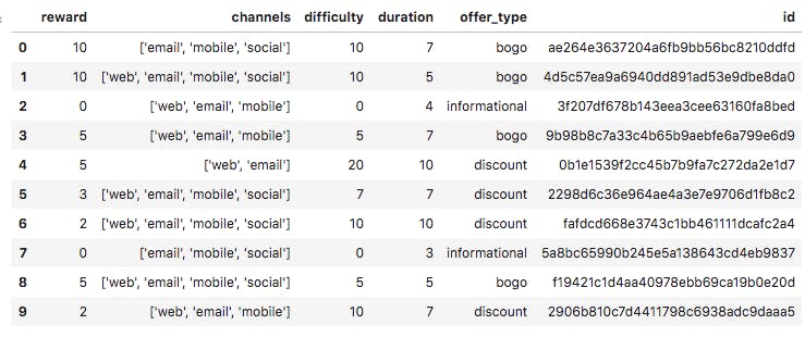
1. Portfolio: This dataset contains details on offers made by Starbucks to its consumers. Size: 10 rows and 6 columns. Features in this dataset include: difficulty (int), reward (int), id (string), offer_type (string), duration (int), channels (list of strings).

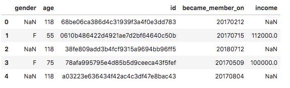
2. Profile: This dataset contains details of customers or consumers of Starbucks’ products. Size: 17000 rows and 5 columns. Features in this dataset include: id (str), age (int), became_member_on (int) gender (str), income (float).

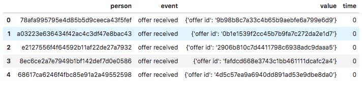
1. Transcript: This dataset contains details on the offers made to consumers of Starbucks’ products. Size: 306534 rows and 4 columns. The Features in this dataset include: event (str), person (str), time (int), value - (dict of strings).

The datasets were obtained by Starbucks and Udacity, as part of the Machine Learning Engineer Capstone Project. The datasets depict the purchase decisions of consumers.

Methodology

Metrics

This project used the following metrics:

1. Confusion Matrix: The confusion matrix detailed the True Positives (TP), False Positives (FP), False Negatives (FN), True Negatives (TN). The purpose of this is to depict the number of correct and wrong predictions made by the model. You can read more on this here

2. Accuracy Score: After this, the model’s accuracy score will be generated. Accuracy measures the ratio of correct predictions over the total number of instances evaluated. Formula for accuracy (TP+TN)/(TP+TN+FP+FN)

Libraries and Packages used in the project

The libraries and/ or packages used for this project include:

-pandas -numpy -matplotlib -seaborn -sklean

Data Cleaning and Processing

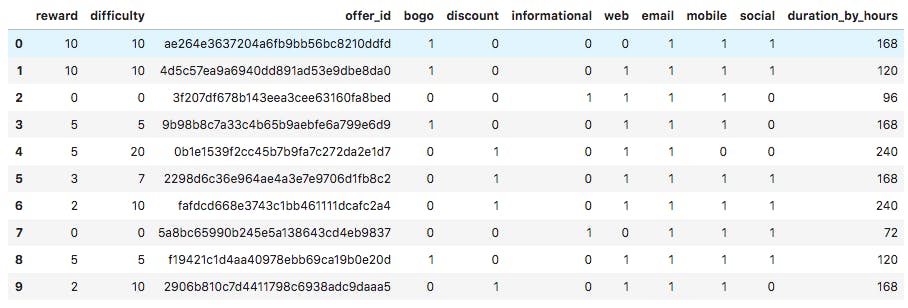
Portfolio Dataset: On the portfolio dataset, the was done to clean and prepare the dataset:

• Renaming the id column to offer_df
• One hot encoding the offer_type column
• Separating the list values in the channels column and one hot encoding them
• Changing the the duration column from days to hours.
• dropping offer_type, duration and channel columns

This is the dataset after cleaning:

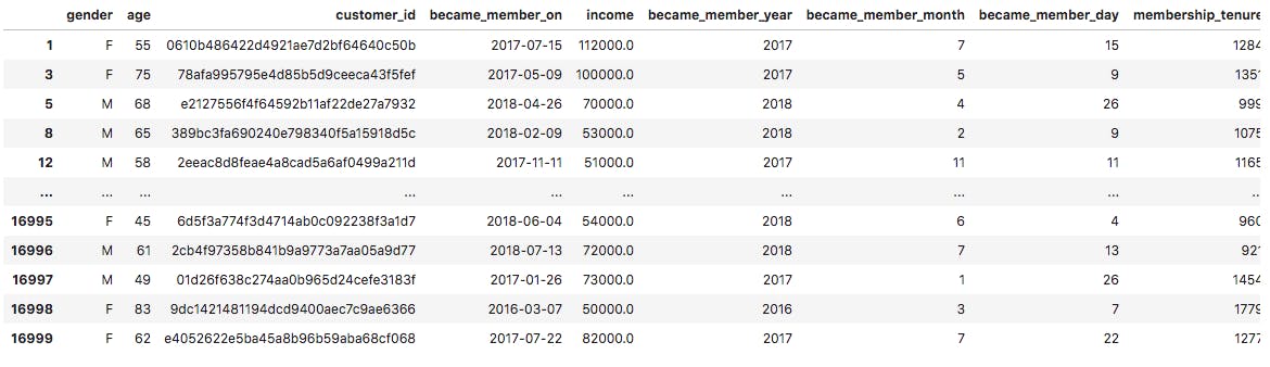
Profile Dataset: the following can be done to clean and prepare the profile dataset:

• Check for and drop null values to a variable
• Transforming the 'became_member_on' column to date format
• Seperating the dates in the 'became_member_on' column into distinct columns: -became_member_year (year) -became_member_month (month) -became_member_day (day)
• Calculating the period the customers have been members
• Creating age_grade column from 'age' column in the profile dataset
• One hot encoding the 'became_member_year', 'became_member_month', 'income_range', 'age_grade' columns
• Renaming the id column to customer_id

This is the cleaned dataset:

Transcript Dataset: The following was done to clean and process the transcript dataset:

• Check for null values
• Change the name of the column from 'Person' to 'customer_id'
• Removing IDs associated with null values in the profile dataset
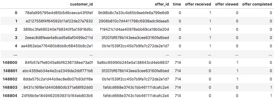
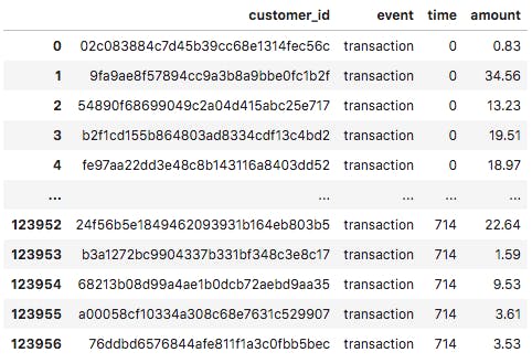
• Separating the dataset into offers_df and transaction_df
• Extracting dict values from the value columns of the newly created datasets to new columns

offers_df: containing data on offers received, viewed and completed

transaction_df: containing data on transactions made

Data Visualisations

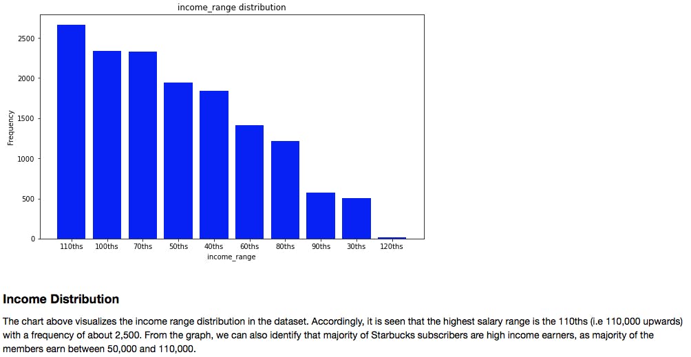
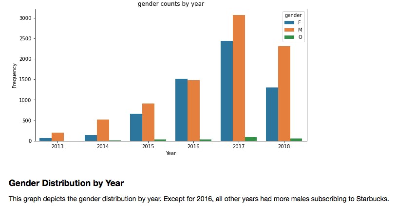
The following were visualised from the profile dataset:

• Income_range Frequency distribution
• Gender distribution by year

Creating a Combined Dataset

Following the cleaning and processing of the three datasets, the next step was combined the datasets into one named combined_df. Combined_df had all the data points represented in the previously cleaned datasets

def create_combined_data(portfolio, profile, offers_df, transaction_df):

    """
    Create a combined dataframe from the transaction, demographic and offer data:
    ARGS:
        portfolio - (dataframe),offer metadata
        profile - (dataframe),customer demographic data
        offers_df - (dataframe), offers data for customers
        transaction_df - (dataframe), transaction data for customers
    """

    combined_data = [] # Initialize empty list for combined data
    customer_id_list = offers_df['customer_id'].unique().tolist() # List of unique customers in offers_df


    # Iterate over each customer
    for i, cust_id in enumerate(customer_id_list):

        # select customer profile from profile data
        cust_profile = clean_profile[clean_profile['customer_id'] == cust_id] 

        # select offers associated with the customer from offers_df
        cust_offers_data = offers_df[offers_df['customer_id'] == cust_id]

        # select transactions associated with the customer from transactions_df
        cust_transaction_df = transaction_df[transaction_df['customer_id'] == cust_id]

        # select received, completed, viewed offer data from customer offers
        offer_received_data  = cust_offers_data[cust_offers_data['offer received'] == 1]
        offer_viewed_data = cust_offers_data[cust_offers_data['offer viewed'] == 1]
        offer_completed_data = cust_offers_data[cust_offers_data['offer completed'] == 1]

        # Iterate over each offer received by a customer
        rows = [] # Initialize empty list for a customer records

        for off_id in offer_received_data['offer_id'].values.tolist():

            # select duration of a particular offer_id
            duration = clean_portfolio.loc[clean_portfolio['offer_id'] == off_id, 'duration_by_hours'].values[0]

            # select the time when offer was received
            off_recd_time = offer_received_data.loc[offer_received_data['offer_id'] == off_id, 'time'].values[0]

            # Calculate the time when the offer ends
            off_end_time = off_recd_time + duration

            #Initialize a boolean array that determines if the customer viewed an offer between offer period
            offers_viewed = np.logical_and(offer_viewed_data['time'] >= off_recd_time,offer_viewed_data['time'] <= off_end_time)

            # Check if the offer type is 'bogo' or 'discount'
            if (clean_portfolio[clean_portfolio['offer_id'] == off_id]['bogo'].values[0] == 1 or\
                    clean_portfolio[clean_portfolio['offer_id'] == off_id]['discount'].values[0] == 1):

                #Initialize a boolean array that determines if the customer completed an offer between offer period
                offers_comp = np.logical_and(offer_completed_data ['time'] >= off_recd_time,\
                                                 offer_completed_data ['time'] <= off_end_time)

                #Initialize a boolean array that selects customer transctions between offer period
                cust_tran_within_period = cust_transaction_df[np.logical_and(cust_transaction_df['time'] >= off_recd_time,\
                                                                                 cust_transaction_df['time'] <= off_end_time)]

                # Determine if the customer responded to an offer(bogo or discount) or not
                cust_response = np.logical_and(offers_viewed.sum() > 0, offers_comp.sum() > 0) and\
                                                    (cust_tran_within_period['amount'].sum() >=\
                                                     clean_portfolio[clean_portfolio['offer_id'] == off_id]['difficulty'].values[0])

            # Check if the offer type is 'informational'
            elif clean_portfolio[clean_portfolio['offer_id'] == off_id]['informational'].values[0] == 1:

                #Initialize a boolean array that determines if the customer made any transctions between offer period
                cust_info_tran = np.logical_and(cust_transaction_df['time'] >= off_recd_time,\
                                                    cust_transaction_df['time'] <= off_end_time)                   

                # Determine if the customer responded to an offer(informational) or not
                cust_response = offers_viewed.sum() > 0 and cust_info_tran.sum() > 0                  

                #Initialize a boolean array that selects customer transctions between offer period
                cust_tran_within_period = cust_transaction_df[np.logical_and(cust_transaction_df['time'] >= off_recd_time,\
                                                                                 cust_transaction_df['time'] <= off_end_time)]

            # Initialize a dictionary for a customer with required information for a particular offer
            cust_rec = {'cust_response': int(cust_response),'time': off_recd_time,'total_amount': cust_tran_within_period['amount'].sum()}
            cust_rec.update(clean_profile[clean_profile['customer_id'] == cust_id].squeeze().to_dict())
            cust_rec.update(clean_portfolio[clean_portfolio['offer_id'] == off_id].squeeze().to_dict())

            # Add the dictionary to list for combined_data
            rows.append(cust_rec)

        # Add the dictionaries from rows list to combined_data list
        combined_data.extend(rows)


    # Convert combined_data list to dataframe
    combined_data_df = pd.DataFrame(combined_data)

    # Reorder columns of combined_data_df
    combined_data_df_col_order = ['customer_id', 'offer_id', 'time']

    port_ls = clean_portfolio.columns.tolist()
    port_ls.remove('offer_id')
    pro_ls = clean_profile.columns.tolist()
    pro_ls.remove('customer_id')
    combined_data_df_col_order.extend(port_ls)
    combined_data_df_col_order.extend(pro_ls)
    combined_data_df_col_order.extend(['total_amount', 'cust_response'])

    combined_data_df = combined_data_df.reindex(combined_data_df_col_order, axis=1)
    combined_data_df.to_csv('combined_data2.csv', index=False)
    return combined_data_df

combined_df = create_combined_data(portfolio, profile, offers_df, transaction_df)
combined_df

In an effort to generate more insights, I created a dataset that showed the amount of offers that were successful.

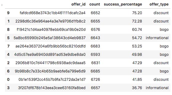
Here is a visualisation of each offer_type and its rate of success (in percentages)

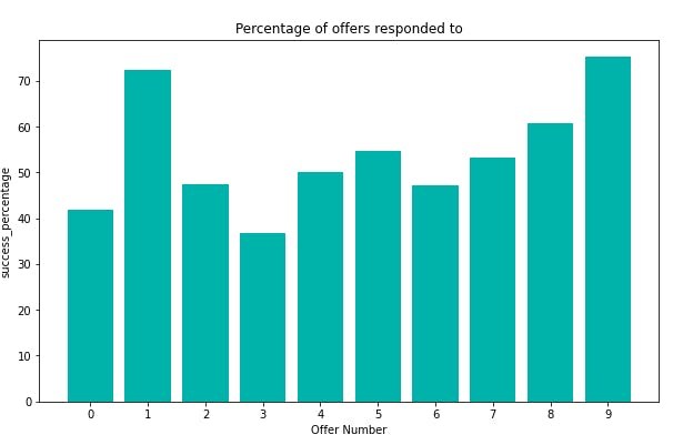
From the preceding, we can see that discount offers are the most successful. Generally, discount and bogo offers out performed informational offers.

Predictive Modelling

Benchmarking

This project adopted a benchmarking approach, by training and testing three distinct classifiers and measuring their performance in terms of their accuracy scores. These classifiers are: Logistic Regression, Random Forest Classifier, Gradient Boosting Classifier. The classifiers were initialised like so:

lr = LogisticRegression(random_state=42) 
rfc = RandomForestClassifier(random_state=42) 
gbc = GradientBoostingClassifier(random_state=42)

Scaling combined_df

In machine learning, it is standard practice that the data is scaled before it can be fed to any model. This is done to optimise performance. The scaling of the dataset was done with the MinMaxScaler() function as initialised above.

Next, I scaled values in the  combined_df dataset. This was done with a scale_features function

#A list of the features we want to scale
features_to_scale = ['difficulty', 'duration_by_hours', 'reward', 'membership_tenure', 'total_amount']

def scale_features(df, feat=features_to_scale):


    """
    This function will scale list features in a given dataframe

    ARGS:
        df (dataframe): dataframe having features to scale
        feat (list): list of features in dataframe to scale
    """

    # Prepare dataframe with features to scale
    df_feat_scale = df[feat]

    # Apply feature scaling to df
    df_feat_scale = pd.DataFrame(scaler.fit_transform(df_feat_scale), columns = df_feat_scale.columns,index=df_feat_scale.index)

    # Drop original features from df and add scaled features 
    df = df.drop(columns=feat, axis=1)
    df_scaled = pd.concat([df, df_feat_scale], axis=1)

    return df_scaled

#Applying the scale_features column to the dataset 
combined_df_scaled = scale_features(combined_df, feat=features_to_scale)

combined_df_scaled

Splitting combined_df_scaled into train and test sets

The scaled data was split into training and testing sets with the train_test_split() as imported above.

# splitting the dataset

# x are the independence variables that act as the input of the model
X = combined_df_scaled.drop(columns=['cust_response'])

# y is the variable to we are trying to predict predict 
y = combined_df_scaled['cust_response']

# split data into train and test sets with train_test_split()
X_train, X_test, y_train, y_test = train_test_split(X, y, test_size=0.3, random_state=42)

The next task was to check the distribution of target values in the y_train set. After running my code, this was the distribution:

1    53.8
0    46.2

From the answer below, we can tell that the training set is almost balanced. It is not extremely imbalanced. As such, no need to worry about dealing with class imbalance.

Training the Classifiers

The three classifiers above were trained simultaneously, with their accuracy scores generated. Here is the code:

def classifier_trainer(X_train, y_train):
    """
    This function trains the identified classifiers with the X_train and y_train sets
    ARGS:
        X_train - Independent variables (Features) training set
        y_train - Dependent variable (Target) training set
        """
    classifiers = [lr, rfc, gbc]
    for classifier in classifiers:
        training = classifier.fit(X_train, y_train)
        score = 'Classifier_Score : {}'.format(classifier.score(X_train, y_train))
        line_breaker = '*****************************'
        print(training)
        print(score)
        print(line_breaker)

#calling the created function on the training sets. 
classifier_trainer(X_train, y_train)

Results:

LogisticRegression(random_state=42)
Classifier_Score : 0.8416111707841031
*****************************
RandomForestClassifier(random_state=42)
Classifier_Score : 0.9999355531686359
*****************************
GradientBoostingClassifier(random_state=42)
Classifier_Score : 0.9114285714285715
*****************************

Testing the Classifiers

The preceding represents the training scores of the identified models. But this is not enough metric to choose a model. The test accuracy score of the models was also needed. The following was done:

def classifier_tester(X_test):
    """
    This function tests the identified classifiers with the X_test set
    ARGS:
        X_test - Independent variables (Features) testing set
        """
    classifiers = [lr, rfc, gbc]
    for classifier in classifiers:
        testing = classifier.predict(X_test)
        score = 'Classifier_test_Score : {}'.format(classifier.score(X_test, y_test))
        line_breaker = '*****************************'
        print(classifier.__class__.__name__)
        print(score)
        print(line_breaker)

classifier_tester(X_test)

Results:

LogisticRegression
Classifier_test_Score : 0.8434664929076237
*****************************
RandomForestClassifier
Classifier_test_Score : 0.9252669039145908
*****************************
GradientBoostingClassifier
Classifier_test_Score : 0.9099794496516466
*****************************

From the training and testing scores above, the Random Forest Classifier out performed the other models with a training and testing accuracy of 0.999 and 0.925 respectively. This happened because of the non-linear nature of the predictions to be made. For more info, please see here. Predictions were made with rfc (Random Forest Classifier) and a confusion matrix was generated to ascertain the True and False predictions.

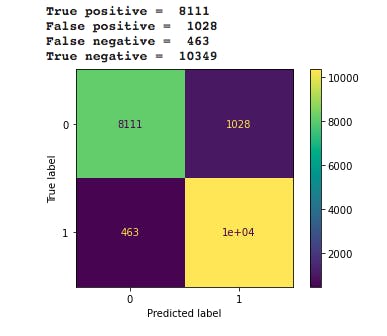
Although the model performed well, false positives and negatives are a bit high. This made tuning necessary. Here is the tuning code used:

clf = RandomForestClassifier(n_estimators=60, criterion='entropy',random_state=42)

clf was used in this case because the Random Forest Classifier was the adopted model.

with the tuned model, new predictions were made and another confusion matrix was generated.

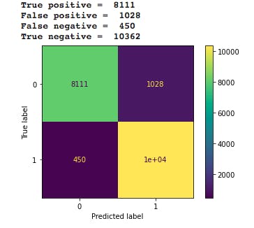
The tuning worked in that it helped reduce the false negative results to 450 from 463 in the initial results. The true negatives also increased from 10349 in the previous confusion matrix, to 10362. These parameters can be changed to get getter results

Results

Following the predictions made, a chart which pictured the most important features in the modelling process. This features are also elements which will inform a customers response to offers made by Starbucks.

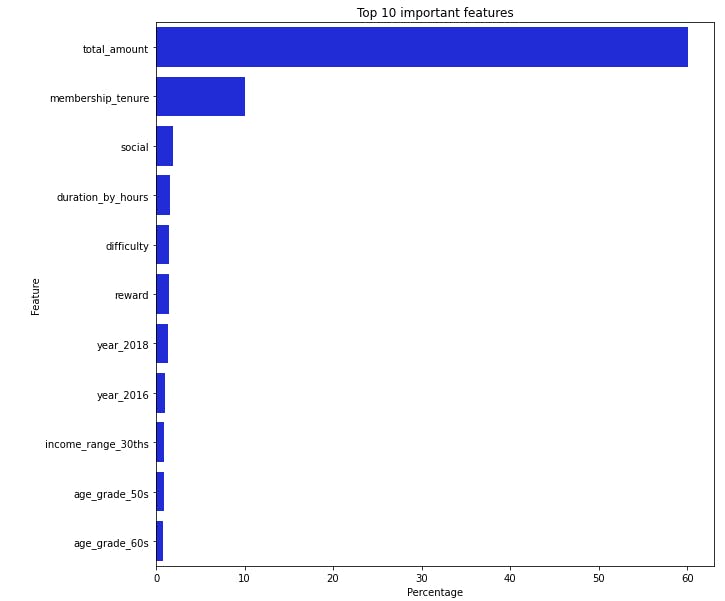
The top four features from the chart above are: total amount, membership tenure, social, difficulty.

• Total Amount: The total amount of money spent by a customer will determine to a large extent, if they will respond to an offer or no

• membership tenure: The membership tenure of customers also determines if they will respond to an offer or not

• social: Social is one of the channels by which customers receive offers. from the visualization above, customers who receved offers through social channels are more likely to respond to offers

• difficulty: difficulty denotes the minimum amount required to be spent before an offer can be completed. The chart shows that difficulty influences a customers decision to respond to an offer or not

Conclusion

The project was set out to determine if a particular customer will respond to an offer or not. Following Data Exploration and Cleaning, the project involved training three classifiers namely: Logistic Regression, Random Forest Classifier and Gradient Boosting Classifier. their scores were measured to determine the model that performs best. with a score of 99% or 0.99, the Random Forest Classifier was chosen and tuned with certain parameters. The predictions were measured with a confusion matrix, to identify the "correct" and "wrong" predictions. With

True positive of 8111, False positive of 1028, False negative of 450, True negative of 10362 it can be said that the model perfomed well. The project also went further to identify the most influential features in the dataset. These features include: total_amount, membership tenure, social and difficulty.

Here is a link to the Github repository, containing the notebook and files used in this project. For enquiries send me a mail: seyiogunnowo@gmail.com

Thank you for reading, i hope you learnt a thing or two